
Data Science is one of the hottest jobs today. According to LinkedIn, the Data Scientist jobs are among the top 10 jobs in the United States. According to The Economic Times, the job postings for the Data Science profile have grown over 400 times over the past one year. So, it is obvious that companies today survive on data, and Data Scientists are the rockstars of this era. So, if you want to start your career as a Data Scientist, you must be wondering what sort of questions are asked in the Data Science interview. So, in this blog, we will be going through Data Science interview questions and answers.
Top Answers to Data Science Interview Questions
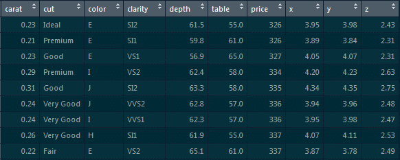
1. From the below given ‘diamonds’ dataset, extract only those rows where the ‘price’ value is greater than 1000 and the ‘cut’ is ideal.
First, we will load the ggplot2 package:
library(ggplot2)
Next, we will use the dplyr package:
library(dplyr)// It is based on the grammar of data manipulation.
To extract those particular records, use the below command:
diamonds %>% filter(price>1000 & cut==”Ideal”)-> diamonds_1000_idea
2. Make a scatter plot between ‘price’ and ‘carat’ using ggplot. ‘Price’ should be on y-axis, ’carat’ should be on x-axis, and the ‘color’ of the points should be determined by ‘cut.’
We will implement the scatter plot using ggplot.
The ggplot is based on the grammar of data visualization, and it helps us stack multiple layers on top of each other.
So, we will start with the data layer, and on top of the data layer we will stack the aesthetic layer. Finally, on top of the aesthetic layer we will stack the geometry layer.
Code:
>ggplot(data=diamonds, aes(x=caret, y=price, col=cut))+geom_point()
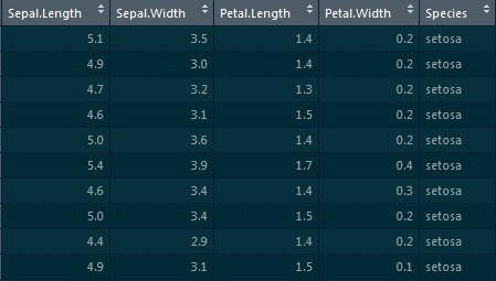
3. Introduce 25 percent missing values in this ‘iris’ datset and impute the ‘Sepal.Length’ column with ‘mean’ and the ‘Petal.Length’ column with ‘median.’
To introduce missing values, we will be using the missForest package:
library(missForest)
Using the prodNA function, we will be introducing 25 percent of missing values:
Iris.mis<-prodNA(iris,noNA=0.25)
For imputing the ‘Sepal.Length’ column with ‘mean’ and the ‘Petal.Length’ column with ‘median,’ we will be using the Hmisc package and the impute function:
library(Hmisc)
iris.mis$Sepal.Length<-with(iris.mis, impute(Sepal.Length,mean))
iris.mis$Petal.Length<-with(iris.mis, impute(Petal.Length,median))
dfdg
4. What do you understand by linear regression?
Linear regression helps in understanding the linear relationship between the dependent and the independent variables.
Linear regression is a supervised learning algorithm, which helps in finding the linear relationship between two variables. One is the predictor or the independent variable and the other is the response or the dependent variable. In Linear Regression, we try to understand how the dependent variable changes w.r.t the independent variable.
If there is more than one independent variable, then it is called simple linear regression, and if there is more than one independent variable then it is known as multiple linear regression.
Interested in learning Data Science? Click here to learn more in this Data Science Training in Sydney!
5. Implement simple linear regression in R on this ‘mtcars’ dataset, where the dependent variable is ‘mpg’ and the independent variable is ‘disp.’
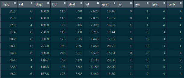
Here, we need to find how ‘mpg’ varies w.r.t displacement of the column.
We need to divide this data into the training dataset and the testing dataset so that the model does not overfit the data.
So, what happens is when we do not divide the dataset into these two components, it overfits the dataset. Hence, when we add new data, it fails miserably on that new data.
Therefore, to divide this dataset, we would require the caret package. This caret package comprises the createdatapartition() function. This function will give the true or false labels.
Here, we will use the following code:
libraray(caret)

split_tag<-createDataPartition(mtcars$mpg, p=0.65, list=F)

mtcars[split_tag,]->train

mtcars[-split_tag,]->test

lm(mpg-data,data=train)->mod_mtcars

predict(mod_mtcars,newdata=test)->pred_mtcars

>head(pred_mtcars)
Explanation:
Parameters of the createDataPartition function: First is the column which determines the split (it is the mpg column).
Second is the split ratio which is 0.65, i.e., 65 percent of records will have true labels and 35 percent will have false labels. We will store this in split_tag object.
Once we have split_tag object ready, from this entire mtcars dataframe, we will select all those records where the split tag value is true and store those records in the training set.
Similarly, from the mtcars dataframe, we will select all those record where the split_tag value is false and store those records in the test set.
So, the split tag will have true values in it, and when we put ‘-’ symbol in front of it, ‘-split_tag’ will contain all of the false labels. We will select all those records and store them in the test set.
We will go ahead and build a model on top of the training set, and for the simple linear model we will require the lm function.
lm(mpg-data,data=train)->mod_mtcars
Now, we have built the model on top of the train set. It’s time to predict the values on top of the test set. For that, we will use the predict function that takes in two parameters: first is the model which we have built and second is the dataframe on which we have to predict values.
Thus, we have to predict values for the test set and then store them in pred_mtcars.
predict(mod_mtcars,newdata=test)->pred_mtcars
Output:
These are the predicted values of mpg for all of these cars.
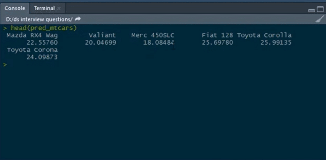
So, this is how we can build simple linear model on top of this mtcars dataset.
6. Calculate the RMSE values for the model built.
When we build a regression model, it predicts certain y values associated with the given x values, but there is always an error associated with this prediction. So, to get an estimate of the average error in prediction, RMSE is used.
Code:
cbind(Actual=test$mpg, predicted=pred_mtcars)->final_data

as.data.frame(final_data)->final_data

error<-(final_data$Actual-final_data$Prediction)

cbind(final_data,error)->final_data

sqrt(mean(final_data$error)^2)
Explanation:
We have the actual and the predicted values. We will bind both of them into a single dataframe. For that, we will use the cbind function:
cbind(Actual=test$mpg, predicted=pred_mtcars)->final_data
Our actual values are present in the mpg column from the test set, and our predicted values are stored in the pred_mtcars object which we have created in the previous question.
Hence, we will create this new column and name the column actual. Similarly, we will create another column and name it predicted which will have predicted values and then store the predicted values in the new object which is final_data.
After that, we will convert a matrix into a dataframe. So, we will use the as.data.frame function and convert this object (predicted values) into a dataframe:
as.data.frame(final_data)->final_data
We will pass this object which is final_data and store the result in final_data again.
We will then calculate the error in prediction for each of the records by subtracting the predicted values from the actual values:
error<-(final_data$Actual-final_data$Prediction)
Then, store this result on a new object and name that object as error.
After this, we will bind this error calculated to the same final_data dataframe:
cbind(final_data,error)->final_data //binding error object to this final_data
Here, we bind the error object to this final_data, and store this into final_data again.
Calculating RMSE:
Sqrt(mean(final_data$error)^2)
Output:
[1] 4.334423
Note: Lower the value of RMSE, the better the model.
R and Python are two of the most important programming languages for Machine Learning Algorithms.
7. Implement simple linear regression in Python on this ‘Boston’ dataset where the dependent variable is ‘medv’ and the independent variable is ‘lstat.’
Simple Linear Regression
import pandas as pd

data=pd.read_csv(‘Boston.csv’)     //loading the Boston dataset

data.head()  //having a glance at the head of this data

data.shape
Let us take out the dependent and the independent variables from the dataset:
data1=data.loc[:,[‘lstat’,’medv’]]

data1.head()
Visualizing Variables
import matplotlib.pyplot as plt

data1.plot(x=’lstat’,y=’medv’,style=’o’)

plt.xlabel(‘lstat’)

plt.ylabel(‘medv’)

plt.show()
Here, ‘medv’ is basically the median values of the price of the houses, and we are trying to find out the median values of the price of the houses w.r.t to the lstat column.
We will separate the dependent and the independent variable from this entire dataframe:
data1=data.loc[:,[‘lstat’,’medv’]]
The only columns we want from all of this record are ‘lstat’ and ‘medv,’ and we need to store these results in data1.
Now, we would also do a visualization w.r.t to these two columns:
import matplotlib.pyplot as plt

data1.plot(x=’lstat’,y=’medv’,style=’o’)

plt.xlabel(‘lstat’)

plt.ylabel(‘medv’)

plt.show()
Preparing the Data
X=pd.Dataframe(data1[‘lstat’])

Y=pd.Dataframe(data1[‘medv’])

from sklearn.model_selection import train_test_split

X_train, X_test, y_train, y_test = train_test_split(X, y, test_size=0.2, random_state=100)

from sklearn.linear_model import LinearRegression

regressor=LinearRegression()

regressor.fit(X_train,y_train)
print(regressor.intercept_)
Output :
34.12654201
print(regressor.coef_)//this is the slope
Output :
[[-0.913293]]
By now, we have built the model. Now, we have to predict the values on top of the test set:
y_pred=regressor.predict(X_test)//using the instance and the predict function and pass the X_test object inside the function and store this in y_pred object
Now, let’s have a glance at the rows and columns of the actual values and the predicted values:
Y_pred.shape, y_test.shape
Output :
((102,1),(102,1))
Further, we will go ahead and calculate some metrics so that we can find out the Mean Absolute Error, Mean Squared Error, and RMSE.
from sklearn import metrics import NumPy as np

print(‘Mean Absolute Error: ’, metrics.mean_absolute_error(y_test, y_pred))

print(‘Mean Squared Error: ’, metrics.mean_squared_error(y_test, y_pred))

print(‘Root Mean Squared Error: ’, np.sqrt(metrics.mean_absolute_error(y_test, y_pred))
Output:
Mean Absolute Error: 4.692198

Mean Squared Error: 43.9198

Root Mean Squared Error: 6.6270
8. What do you understand by logistic regression?
Logistic regression is a classification algorithm which can be used when the dependent variable is binary.
Let’s take an example.
Here, we are trying to determine whether it will rain or not on the basis of temperature and humidity.
Temperature and humidity are the independent variables, and rain would be our dependent variable.
So, logistic regression algorithm actually produces an S shape curve.
Now, let us look at another scenario:
Let’s suppose that x-axis represent the runs scored by Virat Kohli and y-axis represent the probability of team India winning the match. From this graph, we can say that if Virat Kohli scores more than 50 runs, then there is a greater probability for team India to win the match. Similarly, if he scores less than 50 runs then the probability of team India winning the match is less than 50 percent.
So, basically in logistic regression, the y value lies within the range of 0 and 1.
This is how logistic regression works.
9. Implement logistic regression on this ‘heart’ dataset in R where the dependent variable is ‘target’ and the independent variable is ‘age.’
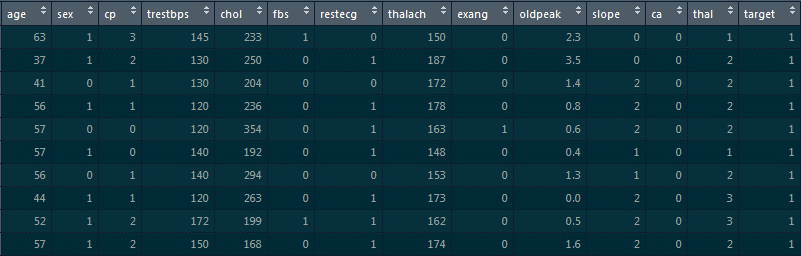
For loading the dataset, we will use the read.csv function:
read.csv(“D:/heart.csv”)->heart

str(heart)
In the structure of this dataframe, most of the values are integers. However, since we are building a logistic regression model on top of this dataset, the final target column is supposed to be categorical. It cannot be an integer. So, we will go ahead and convert them into a factor.
Thus, we will use the as.factor function and convert these integer values into categorical data.
We will pass on heart$target column over here and store the result in heart$target as follows:
as.factor(heart$target)->heart$target
Now, we will build a logistic regression model and see the different probability values for the person to have heart disease on the basis of different age values.
To build a logistic regression model, we will use the glm function:
glm(target~age, data=heart, family=”binomial”)->log_mod1
Here, target~age indicates that the target is the dependent variable and the age is the independent variable, and we are building this model on top of the dataframe.
family=”binomial” means we are basically telling R that this is the logistic regression model, and we will store the result in log_mod1.
We will have a glance at the summary of the model that we have just built:
summary(log_mod1)
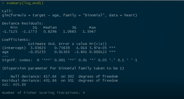
We can see Pr value here, and there are three stars associated with this Pr value. This basically means that we can reject the null hypothesis which states that there is no relationship between the age and the target columns. But since we have three stars over here, this null hypothesis can be rejected. There is a strong relationship between the age column and the target column.
Now, we have other parameters like null deviance and residual deviance. Lower the deviance value, the better the model.
This null deviance basically tells the deviance of the model, i.e., when we don’t have any independent variable and we are trying to predict the value of the target column with only the intercept. When that’s the case, the null deviance is 417.64.
Residual deviance is wherein we include the independent variables and try to predict the target columns. Hence, when we include the independent variable which is age, we see that the residual deviance drops. Initially, when there are no independent variables, the null deviance was 417. After we include the age column, we see that the null deviance is reduced to 401.
This basically means that there is a strong relationship between the age column and the target column and that is why the deviance is reduced.
As we have built the model, it’s time to predict some values:
predict(log_mod1, data.frame(age=30), type=”response”)

predict(log_mod1, data.frame(age=50), type=”response”)

predict(log_mod1, data.frame(age=29:77), type=”response”)
Now, we will divide this dataset into train and test sets and build a model on top of the train set and predict the values on top of the test set:
>library(caret)

Split_tag<- createDataPartition(heart$target, p=0.70, list=F)

heart[split_tag,]->train

heart[-split_tag,]->test

glm(target~age, data=train,family=”binomial”)->log_mod2

predict(log_mod2, newdata=test, type=”response”)->pred_heart

range(pred_heart)
10. What is a confusion matrix?
Confusion matrix is a table which is used to estimate the performance of a model. It tabulates the actual values and the predicted values in a 2×2 matrix.
True Positive (d): This denotes all of those records where the actual values are true and the predicted values are also true. So, these denote all of the true positives.
False Negative (c): This denotes all of those records where the actual values are true, but the predicted values are false.
False Positive (b): In this, the actual values are false, but the predicted values are true.
True Negative (a): Here, the actual values are false and the predicted values are also false.
So, if you want to get the correct values, then correct values would basically represent all of the true positives and the true negatives.
This is how confusion matrix works.
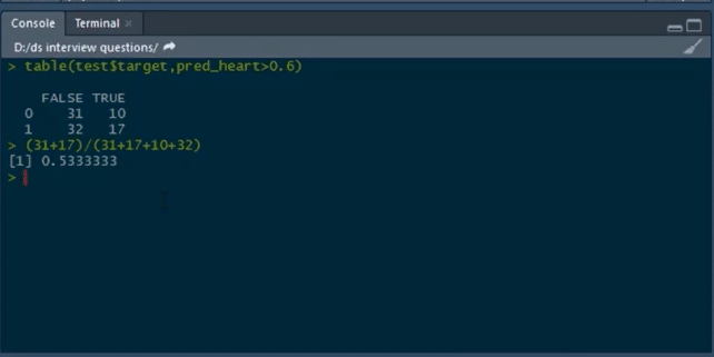
11. Build a confusion matrix for the model where the threshold value for the probability of predicted values is 0.6, and also find the accuracy of the model.
Accuracy is calculated as:
Accuracy = (True positives + true negatives)/(True positives+ true negatives + false positives + false negatives)
To build a confusion matrix in R, we will use the table function:
table(test$target,pred_heart>0.6)
Here, we are setting the probability threshold as 0.6. So, wherever the probability of pred_heart is greater than 0.6, it will be classified as 0, and wherever it is less than 0.6 it will be classified as 1.
Then, we calculate the accuracy by the formula for calculating Accuracy.
Learn more about Data Cleaning in Data Science Tutorial!
12. What do you understand by true positive rate and false positive rate?
True positive rate: In Machine Learning, true positives rates, which are also referred to as sensitivity or recall, are used to measure the percentage of actual positives which are correctly indentified.
Formula: True Positive Rate = True Positives/Positives
False positive rate: False positive rate is basically the probability of falsely rejecting the null hypothesis for a particular test. The false positive rate is calculated as the ratio between the number of negative events wrongly categorized as positive (false positive) upon the total number of actual events.
Formula: False Positive Rate = False Positives/Negatives
Check out this comprehensive Data Science Course!
13. What is ROC curve?
It stands for Receiver Operating Characteristic. It is basically a plot between a true positive rate and a false positive rate, and it helps us to find out the right tradeoff between the true positive rate and the false positive rate for different probability thresholds of the predicted values. So, the closer the curve to the upper left corner, the better the model is. In other words, whichever curve has greater area under it that would be the better model.
You can see this in the below graph:
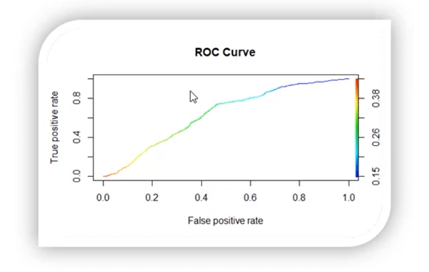
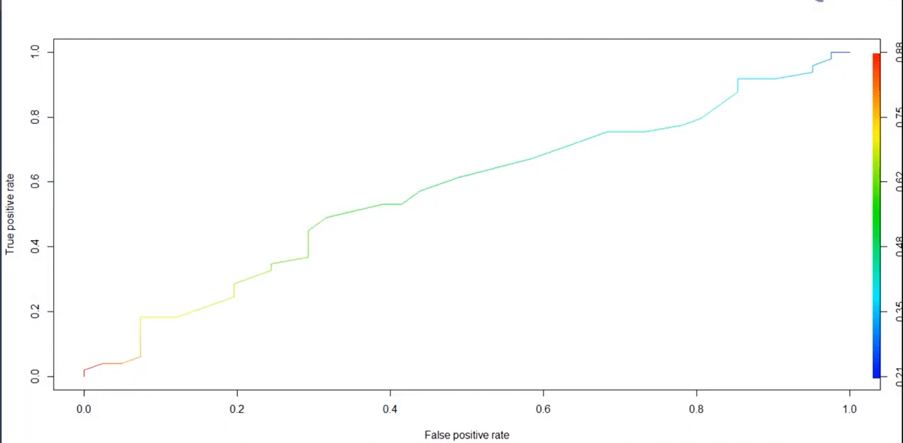
14. Build an ROC curve for the model built.
The below code will help us in building the ROC curve:
library(ROCR)

prediction(pred_heart, test$target)-> roc_pred_heart

performance(roc_pred_heart, “tpr”, “fpr”)->roc_curve

plot(roc_curve, colorize=T)
Graph:
Go through this Data Science Course in London to get a clear understanding of Data Science!
15. Build a logistic regression model on the ‘customer_churn’ dataset in Python. The dependent variable is ‘Churn’ and the independent variable is ‘MonthlyCharges.’ Find the log_loss of the model.
First, we will load the pandas dataframe and the customer_churn.csv file:
customer_churn=pd.read_csv(“customer_churn.csv”)
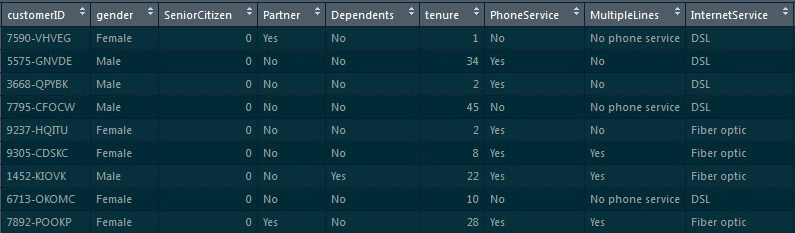
After loading this dataset, we can have a glance at the head of the dataset by using the following command:
customer_churn.head()
Now, we will separate the dependent and the independent variables into two separate objects:
x=pd.Dataframe(customer_churn[‘MonthlyCharges’])

y=customer_churn[‘ Churn’]

#Splitting the data into training and testing sets

from sklearn.model_selection import train_test_split

x_train, x_test, y_train, y_test=train_test_split(x,y,test_size=0.3, random_state=0)
Now, we will see how to build the model and calculate log_loss.
from sklearn.linear_model, we have to import LogisticRegression

l=LogisticRegression()

l.fit(x_train,y_train)

y_pred=l.predict_proba(x_test)
As we are supposed to calculate the log_loss, we will import it from sklearn.metrics:
from sklearn.metrics import log_loss

print(log_loss(y_test,y_pred)//actual values are in y_test and predicted are in y_pred
Output:
0.5555020595194167
Become a master of Data Science by going through this online Data Science Course in Toronto!
16. What do you understand by a decision tree?
A decision tree is a supervised learning algorithm that is used for both classification and regression. Hence, in this case, the dependent variable can be both a numerical value and a categorical value.
Here, each node denotes the test on an attribute, and each edge denotes the outcome of that attribute, and each leaf node holds the class label.
So, in this case, we have a series of test conditions which gives the final decision according to the condition.
Are you interested in learning Data Science from experts? Enroll in our Data Science Course in Bangalore now!
17. Build a decision tree model on ‘Iris’ dataset where the dependent variable is ‘Species,’ and all other columns are independent variables. Find the accuracy of the model built.
To build a decision tree model, we will be loading the party package:
#party package

library(party)

#splitting the data

library(caret)

split_tag<-createDataPartition(iris$Species, p=0.65, list=F)

iris[split_tag,]->train

iris[~split_tag,]->test

#building model

mytree<-ctree(Species~.,train)
Now we will plot the model
plot(mytree)
Model:
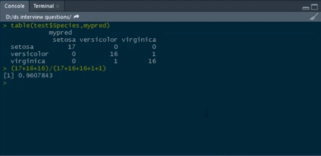
#predicting the values

predict(mytree,test,type=’response’)->mypred
After this, we will predict the confusion matrix and then calculate the accuracy using the table function:
table(test$Species, mypred)
To learn Data Science from experts, click here Data Science Training in New York!
18. What do you understand by a random forest model?
It combines multiple models together to get the final output or, to be more precise, it combines multiple decision trees together to get the final output. So, decision trees are the building blocks of the random forest model.
19. Build a random forest model on top of this ‘CTG’ dataset, where ‘NSP’ is the dependent variable and all other columns are independent variables.
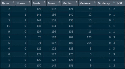
We will load the CTG dataset by using read.csv:
data<-read.csv(“C:/Users/intellipaat/Downloads/CTG.csv”,header=True)

str(data)
Converting the integer type to a factor
data$NSP<-as.factor(data$NSP)

table(data$NSP)

#data partition

set.seed(123)

split_tag<-createDataPartition(data$NSP, p=0.65, list=F)

data[split_tag,]->train

data[~split_tag,]->test

#random forest -1

library(randomForest)

set.seed(222)

rf<-randomForest(NSP~.,data=train)

rf

#prediction

predict(rf,test)->p1
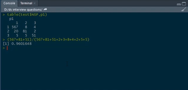
Building confusion matrix and calculating accuracy:
table(test$NSP,p1)
If you have any doubts or queries related to Data Science, get them clarified from Data Science experts on our Data Science Community!
20. How is Data modeling different from Database design?
Data Modeling: It can be considered as the first step towards the design of a database. Data modeling creates a conceptual model based on the relationship between various data models. The process involves moving from the conceptual stage to the logical model to the physical schema. It involves the systematic method of applying data modeling techniques.
Database Design: This is the process of designing the database. The database design creates an output which is a detailed data model of the database. Strictly speaking, database design includes the detailed logical model of a database but it can also include physical design choices and storage parameters.
Related course
Mastering Python – Machine Learning
Learn Internet of Things (IoT) Programming
Oracle BI – Create Analyses and Dashboards
Microsoft Power BI with Advance Excel

Leave a Reply